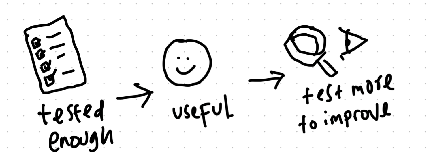
When can we say that a software is tested "enough"?
The principles and technique to help understand when test coverage can be considered as "enough".
You’re building a very important feature for your customers. You know that a defect found by your customer in your software will hurt their trust in your product so you wanted to be very careful about this, but how do you know that you’ve tested enough?
This post aims to answer that question, especially for functional black-box testing.
The seven testing principles
First of all, let’s take a look at the seven testing principles that are introduced by the International Software Testing Qualification Board (ISTQB). According to ISTQB, the principles “offer general guidelines common for all testing.”
This will be our foundation in understanding what is considered enough coverage for testing:
| Principle | Meaning |
|---|---|
| Testing is context dependent | Testing is done differently in different contexts, safety-critical software will be tested differently from e-commerce, so keep in mind of the context when testing. |
| Exhaustive testing is impossible | It is not feasible to test every single possible cases except for trivial cases, so you need to use risk analysis, test techniques, and priorities should be used to focus test efforts. |
| Defects cluster together | A small number of modules usually contains most of the defects, predicting it is an important input into a risk analysis used to focus the test effort. |
| Testing shows the presence of defects, not their absence | Because it is costly to test everything, testing is a mechanism to show the presence of defect and can NOT prove absence of defect nor that the software is correct. |
| Early testing saves time and money | It is better to detect defect early as it helps reduce or eliminate costly changes. |
| Beware of the pesticide paradox | Repeating the same set of tests will not uncover new defects so test data may need changing and new tests may need to be added. |
| Absence-of-errors is a fallacy | Despite all the test, a defect-free software is still an unusable software if it does NOT follow the user's requirements. |
For this post, I intentionally changed the sequence and rephrased the meaning of the principles so that it is easier to understand them all cohesively—so try reading only the meaning from top to bottom.
If you’d like to, you can see them yourself from the original document from ISTQB.
Now you can see that we can surmise the criteria of what is “enough coverage” as below:
- There is no other meaningful test that can be run (redundancy-free), judged by doing risk assessment and testing techniques
- The software can be considered as usable by the user
- Tests are made with the software’s context in mind:
- the environment (such as viewport, OS, hardware, etc.)
- the user (such as tech-saviness, while multi-tasking, low internet connection, etc.)
The testing techniques
Testing techniques are tools to help us cover enough testing ground. These techniques are generally made to reduce redundancy in tests and focus on areas where the defects are most likely to happen.
Note that the techniques listed below are by no means exhaustive, but only a handful that I have learned and understand so far. I will add more over time.
Just like all other tools, no one tool is right and each shall be applied—solely or in combination with another—accordingly.
Equivalence Partitioning
This technique splits data into multiple valid and invalid partitions that are expected to be processed in the same way and makes a test case from the value in each of the partitions. It ensures that each condition is tested at least once.
Valid partitions should contain values that are accepted by the system, while invalid partitions are values rejected by the system.
The technique considers 100% coverage when all partitions are tested by at least one value from each partition.
The technique works better for data with discrete values. Check the Boundary Value Analysis technique for work with sequential or numerical range data.
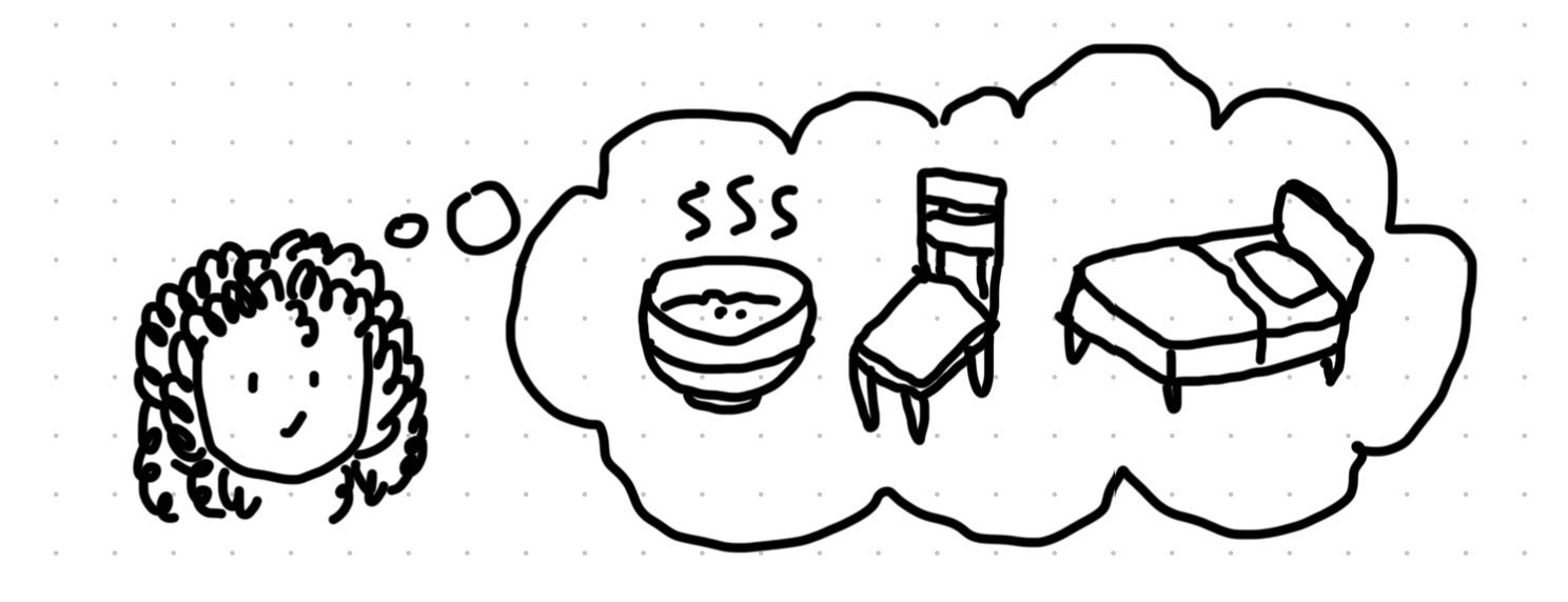
INTERESTING THOUGHT
In the fairy tale Goldilocks and the Three Bears, Goldilocks uses similar technique to this when trying the three bear’s properties:
Papa bear’s Son bear’s Mama bear’s invalid valid invalid Porridge too hot just right too cold Chair too hard just right too delicate Bed too hard just right too delicate
Example
Customer will get:
- 5% discount for $1–10 purchase
- 10% discount for $11–100 purchase
- 15% discount for above
Minimum purchase is $1 and maximum is $500
Instead of testing sporadically and without knowing if the condition is tested enough …
- $6 should get a 5% discount
- $10 should get a 5% discount
- $13 should get a 10% discount
- $34 should get a 10% discount
- $88 should get a 10% discount
- $120 should get a 15% discount
- $400 should get a 15% discount
… the technique allows clarity in defining “enough” by demanding exactly 5 tests to ensure all conditions are tested:
- $0.5 should be invalid
- $6 should get a 5% discount
- $34 should get a 10% discount
- $400 should get a 15% discount
- $700 should be invalid
Step by step
Let’s use the sample above:
Valid input is only letters and not symbols nor numbers
-
Turn the conditional statement into valid and invalid partitions.
invalid valid invalid type symbols letters numbers range ~!@#?/… A to z 0 to 9 -
Take a value from each partition as a test case
- ’$’ should result in invalid
- ‘F’ should get 5% discount
- ‘4’ should result in invalid
Boundary Value Analysis
Most often, the defect of a numeric range or sequential data can be found on its edges rather than the middle value. This technique is an extension of the Equivalence Partitioning technique that focuses on those edges to make sure the boundaries are set correctly as values on the boundaries are more prone to defect than ones that are within.
In this context, each partition will have valid values and invalid values.
The technique considers 100% coverage if all valid and invalid values for all partitions are tested at least once.
Example
Customer will get:
- 5% discount for $1–10 purchase
- 10% discount for $11–100 purchase
- 15% discount for above
Which resulted in these 6 test cases:
- $0 should be no discount
- $1 should get a 5% discount
- $10 should get a 5% discount
- $11 should get a 10% discount
- $100 should get a 10% discount
- $101 should get a 15% discount
Step by step
Let’s use the sample above:
Valid input is only letters and not symbols nor numbers
-
Turn the conditional statement into valid and invalid partitions.
discount 0% 5% 10% 15% range < $1 < $11 < 101 > $101 -
Take valid and invalid values on the edge of each partition
- partition 0%:
- invalid: -$0.01
- valid: $0
- valid: $0.99
- invalid: $1
- partition 5%:
- invalid: $0.99
- valid: $1
- valid: $10.99
- invalid: $11
- partition 10%:
- invalid: $10.99
- valid: $11
- valid: $100.99
- invalid: $101
- partition 15%:
- invalid: $100.99
- valid: $101
- partition 0%:
-
Combine and remove the redundant tests
- -$0.01 should be rejected
- $0 should get no discount
- $0.99 should get no discount
- $1 should get a 5% discount
- $10.99 should get a 5% discount
- $11 should get a 10% discount
- $100.99 should get a 10% discount
- $101 should get a 15% discount
Decision Table
Also called the “Cause Effect Table” because it maps a system’s effects and its causes. Laying down each variable and its states (boolean or discrete) alongside the effect it causes.
This is best used to record and test complex business rules that a system must implement.
The technique considers 100% coverage when all the decision rule is covered. Note that the strength of this technique lies in making sure no decisions are left untested, so this may a huge number of cases need to be created and run.
Example
Registration form that asked for email, and password.
| Test case | 1 | 2 | 3 | 4 | 5 |
|---|---|---|---|---|---|
| Conditions | |||||
| Y | Y | N | Y | N | |
| Password | Y | Y | Y | N | N |
| Effects | |||||
| Success message | Y | Y | N | N | N |
| Error message | N | N | Y | Y | Y |
Step by step
Let’s use this as an example:
Test a registration form that:
- requires a valid email
- requires a valid password which is 8 or more charactes and is a combination of numbers and letters
- optional opt-in to newsletter communication via email
-
List down the conditions and possible effects that may happen—make sure to list down the effect rather than putting it in the table to make it easier to comprehend
Test case Conditions Email Password (8 char with numbers & letters) Password (8 char, only numbers) Password (8 char, only letters) Password (7 char with numbers & letters) Newsletter opt-in Effects Success message Error message Send welcoming newsletter -
Jot down the different conditions that are met as well as their appropriate effects; you may use:
- ‘Y’ or ‘N’ to represent ‘Yes’ or ‘No’,
- ‘T’ or ‘F’ to represent ‘True’ or ‘False’,
- ‘1’ or ‘0’ to represent boolean,
- the discrete value (such as “red”, “green”, “XXL”, etc.) if that is the data type requested, or
- ’-‘ if not relevant
Test case 1 2 3 4 5 6 7 8 Conditions Email Y Y N Y Y Y Y N Password (8 char with numbers & letters) Y Y Y N - - - N Password (8 char, only numbers) - - - - Y - - - Password (8 char, only letters) - - - - - Y - - Password (7 char with numbers & letters) - - - - - - Y - Newsletter opt-in Y N - - - - - - Effects Success message Error message Send welcoming newsletter -
Jot down the respective effects given the conditions you’ve listed; which can be expressed by:
- Use ‘X’, ‘Y’, ‘T’, or ‘1 to mark that an action should occur, and
- Blank (preferable for ease of reading), ‘N’, ‘F’, or ‘0’ to indicate the action will not occur.
- It is also okay to put a specific message shown in or beside the table if relevant.
Test case 1 2 3 4 5 6 7 8 Conditions Email Y Y N Y Y Y Y N Password (8 char with numbers & letters) Y Y Y N - - - N Password (8 char, only numbers) - - - - Y - - - Password (8 char, only letters) - - - - - Y - - Password (7 char with numbers & letters) - - - - - - Y - Newsletter opt-in Y N - - - - - - Effects Success message X X Error message X-1 X-2 X-2 X-2 X-2 X-2 Send welcoming newsletter X X Notes
- Success message: “Your account has been successfully created!”
- Error messages:
- “Email is required.”
- “Password must contain 8 or more characters and is a combination of number and letter.”
Pairwise
The technique is based on the observation that most faults are caused by interactions of at most two factors. It significantly reduces the amount of test needed simply by making sure a pair of each test are only tested once whenever possible.
This is best applied to settings or configurational features.
The technique considers 100% coverage when all variable value pairs are represented in a test at least once.
Example
Format method: quick, slow
File system:   FAT, FAT32, NTFS
Compression:   on, off
Instead of doing all 12 combinations to test …
quick + FAT + onquick + FAT + offquick + FAT32 + onquick + FAT32 + offquick + NTFS + onquick + NTFS + offslow + FAT + onslow + FAT + offslow + FAT32 + onslow + FAT32 + offslow + NTFS + onslow + NTFS + off
… the technique allows us to only do 6 tests with a high degree of confidence since all variables’ values are paired at least once with another variable’s value. That is a 50% decrease.
quick + FAT + onquick + FAT32 + offslow + FAT + offslow + FAT32 + onquick + NTFS + onslow + NTFS + off
A bigger set of combinations will result in a bigger efficiency. For example, the combination below has 4,704 combinations, only 62 are needed when using the Pairwise technique. That is a whopping 98.6% decrease!
Type:          Primary, Logical, Single, Span, Stripe, Mirror, RAID-5
Size:          10, 100, 500, 1000, 5000, 10000, 40000
Format method: quick, slow
File system:   FAT, FAT32, NTFS
Cluster size:  512, 1024, 2048, 4096, 8192, 16384, 32768, 65536
Compression:   on, off
Primary + 10 + slow + FAT32 + 16384 + onPrimary + 100 + quick + FAT + 2048 + offPrimary + 100 + quick + NTFS + 512 + offPrimary + 500 + quick + FAT + 65536 + offPrimary + 500 + slow + FAT32 + 4096 + offPrimary + 1000 + slow + FAT + 1024 + onPrimary + 5000 + quick + NTFS + 1024 + offPrimary + 10000 + slow + FAT + 32768 + onPrimary + 40000 + slow + FAT + 8192 + onPrimary + 40000 + quick + NTFS + 32768 + onLogical + 500 + quick + NTFS + 8192 + offLogical + 10000 + slow + NTFS + 512 + offLogical + 40000 + quick + FAT32 + 16384 + offLogical + 10 + quick + FAT + 2048 + onLogical + 100 + quick + NTFS + 32768 + offLogical + 1000 + slow + FAT + 4096 + offLogical + 10000 + slow + NTFS + 1024 + offLogical + 5000 + slow + NTFS + 65536 + offLogical + 10000 + quick + FAT + 4096 + offSingle + 10 + quick + FAT + 512 + offSingle + 10000 + quick + FAT32 + 65536 + offSingle + 100 + quick + FAT + 8192 + onSingle + 5000 + quick + NTFS + 16384 + offSingle + 10 + quick + NTFS + 4096 + onSingle + 1000 + slow + FAT32 + 2048 + offSingle + 40000 + quick + FAT + 1024 + offSingle + 500 + quick + FAT32 + 512 + offSingle + 5000 + quick + FAT + 32768 + onSpan + 5000 + slow + FAT32 + 2048 + onSpan + 10000 + slow + FAT + 16384 + onSpan + 1000 + quick + NTFS + 512 + onSpan + 10 + slow + FAT32 + 32768 + offSpan + 500 + slow + FAT + 1024 + offSpan + 40000 + quick + FAT + 4096 + onSpan + 100 + quick + FAT + 65536 + onSpan + 1000 + quick + NTFS + 65536 + offSpan + 5000 + slow + FAT + 8192 + offStripe + 100 + quick + FAT32 + 1024 + onStripe + 5000 + slow + NTFS + 32768 + onStripe + 5000 + quick + FAT + 4096 + offStripe + 500 + quick + NTFS + 16384 + onStripe + 10000 + quick + FAT32 + 512 + offStripe + 40000 + quick + FAT32 + 65536 + onStripe + 1000 + quick + FAT + 8192 + offStripe + 10 + quick + NTFS + 2048 + offMirror + 1000 + quick + FAT + 32768 + offMirror + 100 + slow + NTFS + 65536 + onMirror + 10 + quick + FAT32 + 8192 + offMirror + 500 + quick + FAT32 + 2048 + onMirror + 5000 + quick + FAT + 512 + onMirror + 10000 + slow + FAT + 2048 + offMirror + 40000 + slow + FAT32 + 4096 + offMirror + 10 + slow + FAT32 + 1024 + offMirror + 100 + slow + FAT32 + 16384 + offRAID-5 + 500 + slow + FAT + 32768 + onRAID-5 + 100 + slow + FAT32 + 4096 + offRAID-5 + 40000 + quick + NTFS + 2048 + onRAID-5 + 5000 + quick + NTFS + 1024 + onRAID-5 + 10000 + slow + NTFS + 8192 + onRAID-5 + 1000 + quick + FAT + 16384 + onRAID-5 + 10 + slow + FAT32 + 65536 + offRAID-5 + 40000 + quick + FAT32 + 512 + on
Step by step
The simplest way is, of course, to use a generator. One that I found incredibly easy to use is the Pairwise Independent Combinatorial Testing (PICT) tool which is a FOSS made by Microsoft.
But if you’d like to do it manually, I’ll guide you on the step by step on how to do it using this as a context:
We need to test our system works well on any of the following configuration:

Format method: quick, slow
File system:   FAT, FAT32, NTFS
Compression:   on, off
-
You make a pair for each variable, making sure all pair combinations are made.
quick + FATquick + FAT32quick + NTFSquick + onquick + offslow + FATslow + FAT32slow + NTFSslow + onslow + offFAT + onFAT + offFAT32 + onFAT32 + offNTFS + onNTFS + off
-
Arrange a combination of all 3 sequences using all available pairs
quick + FAT + on–>quick + FAT&FAT + on&quick + onquick + FAT32 + off—>quick + FAT32&FAT32 + off&quick + offslow + FAT + off–>slow + FAT&FAT + off&slow + offslow + FAT32 + on–>slow + FAT32&FAT32 + on&slow + onquick + NTFS + on–>quick + NTFS&NTFS + on& redundancy ofquick + onslow + NTFS + off–>slow + NTFS&NTFS + off& redundancy ofslow + off
-
As you can see, the last two on the list have a repeat combination of
quick + onandslow + off, but since this is inevitable, this is a necessary redundancy.
Concluding thoughts
Here are the key takeaways from the above.
- No software can be defect-free as it is not viable, so tests should be done just enough to make you confident that it is stable and reliable enough before releasing it to the user
- There are testing techniques that help you get an idea of how much can be considered just enough such as:
- Equivalence partitioning, ensures all valid and invalid conditions are tested.
- Boundary Value Analysis, ensure boundaries between value ranges are properly established.
- Decision Table, ensure no decision rules are left untested.
- Pairwise, for combinatorial values.
An additional point to make from my reflection is that, the technique helps us understand what is “enough”, but as the principle said, once it is more stable, it is wise to add more tests to uncover more defects—keeping in mind that a usable software is more important than a fully defect-free software.
Relevant references
- The seven testing principles and some of the testing techniques can be found on ISTQB’s Foundation Level (CTFL) Syllabus
- Well-written description of the seven testing principles by Box UK
- Pairwise Independent Combinatorial Testing (PICT) tool, a FOSS tool to generate Pairwise tests by Microsoft:
- Good explanation video by Software Testing Mentor on YouTube:
End-notes
This post is dedicated to Yustika and Kocoy, the QEs from my previous startup, Farmacare.